Visualizing Core ideas

Core idea

A model suite (here 500M, 1.5B and 3B parameters) is normally three separate training runs. Godey and Artzi (2026) instead stack the models into one: the 500M model is the first block of the network, the 1.5B model is the first two blocks, and the 3B model is all three. One run trains every size, and each smaller model can still be cut out and served on its own.

The paper spreads this idea across several places. Section 2 gives the nesting and the exits. Equation 1 defines the junction that connects one block to the next. Equations 2 and 3 define the distillation loss, in which the largest exit teaches the smaller ones. Table 1 gives the layer counts, widths and parameter totals. Figure 1(a) draws the nesting but not the mechanism. A new reader has to combine all of these to see why the design works and why it is cheaper, so this figure puts them in one place.

The figure

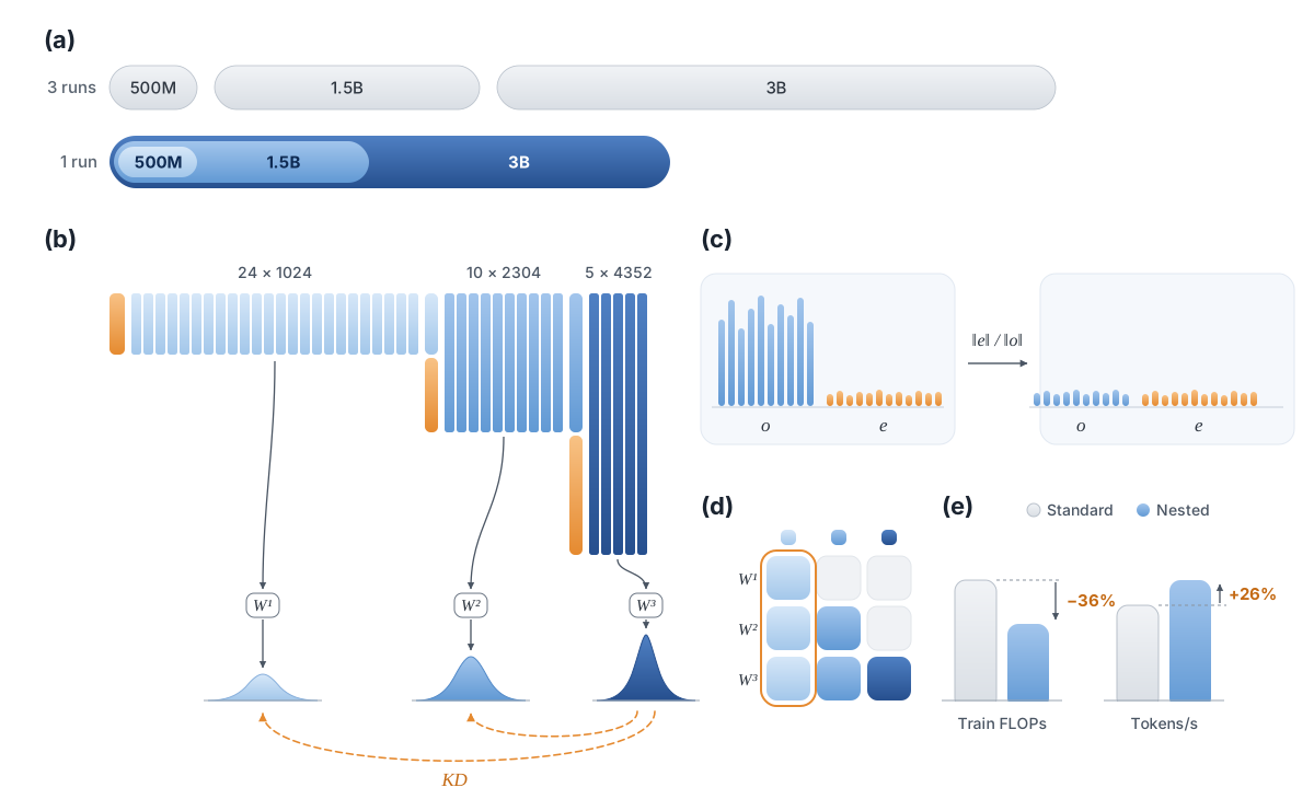
Accuracy is not in the figure. The paper reports it within 0.5 average points of token-matched baselines at every size, and those baselines use 57% more compute.

How to read it and why it is drawn this way

• (a) What is nested. The top row is a standard suite of three models. The bottom row nests the 500M, 1.5B and 3B bars inside each other, with widths proportional to the paper’s parameter counts (3.2B for the nested suite against 5.2B).
• (b) How it is built. Bar heights follow the paper’s block widths (1024, 2304, 4352) and layer counts (24, 10, 5), so you can see why the later blocks are wide and short. Orange strips are fresh embedding channels. Each block ends in an exit with its own LM head, and the dashed arrows show distillation from the 3B exit into the smaller ones, and only into them, because the paper defines the distillation term only for the smaller exits.
• (c) How the blocks connect. The junction is the paper’s one new component and exists in the text only as an equation. The output of one block is much larger than a fresh embedding, so it is rescaled to the embedding’s norm and the two are concatenated. It adds no parameters. In the paper’s 200M ablation, dropping the rescaling costs about 0.2 validation perplexity, and replacing the fresh embedding with zeros costs about 0.54.
• (d) Who trains what. Rows are exits and columns are blocks, so it is visible at once that block 1 is trained by all three losses. That is why it has to work as a standalone 500M model and as the start of the larger ones.
• (e) What it saves. The 36% is training compute (7.0e21 vs. about 1.1e22 FLOPs). The 26% is greedy speculative decoding at draft length 6, 2,650 vs. 2,100 tokens/s against an independently trained pair.
• One colour system. The blue ramp marks blocks in every panel, and orange marks fresh embedding channels and distillation.

Two caveats on the numbers. The paper’s 3.2B vs. 5.2B parameter count leaves out the LM heads of the two smaller exits, which add about 0.16B. And part of the decoding speedup comes from a larger batch fitting in memory (102 vs. 64), because the draft shares the verifier’s KV cache.