Visualizing the core idea of Matryoshka LM Suites

Core idea:

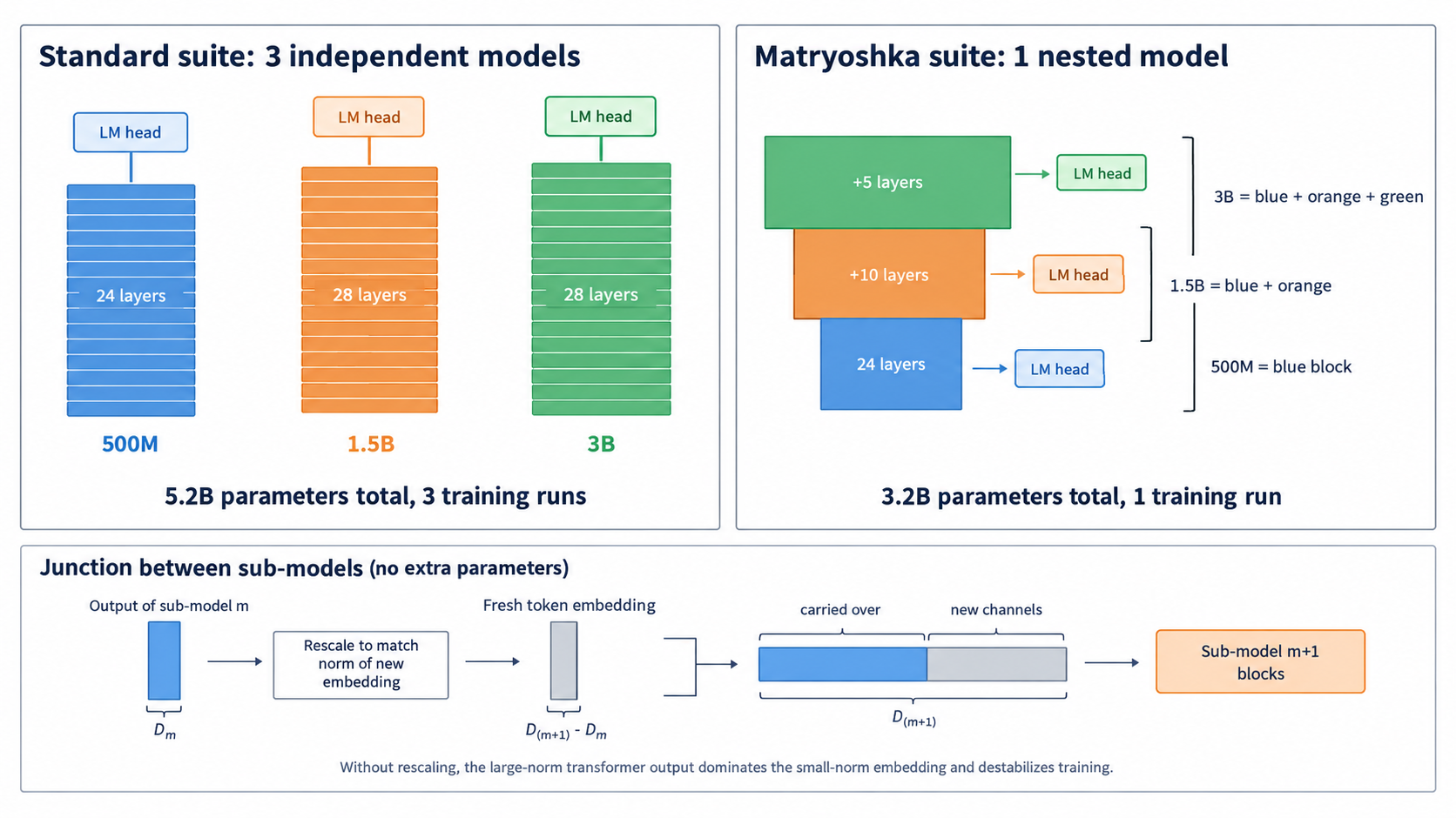
The core idea of the paper (Godey and Artzi, 2026) is explained in Section 2 and in Figure 1(a). A model suite is a group of models of different sizes, here 500M, 1.5B and 3B parameters. Usually, each model is trained separately. The paper builds one model in which the small models are contained inside the large one. The first 24 layers form the 500M model, 10 more layers extend it to the 1.5B model, and 5 more layers extend it to the 3B model. Each size has its own output layer (LM head), and all sizes are trained together in a single run. The result is a complete suite from one training run, with fewer parameters in total (3.2B instead of 5.2B).

The idea is hard to see in the paper, because it is spread over three places. The structure (which layers are shared between the sub-models) is in the text of Section 2. The mechanism that connects the sub-models, the junction, appears only in Equation 1. The numbers behind the savings are in Table 1. A new reader has to combine all three to understand why this works and why it is cheaper.

The figure:

How to read it.

• Left panel: a standard suite. Three independent models, each with its own embedding and LM head, trained in three separate runs. The total is 5.2B parameters.
• Right panel: a Matryoshka suite. One stack of three blocks (24, +10 and +5 layers). The blue block is exactly the 500M model. Blue plus orange is the 1.5B model. All three blocks together are the 3B model. Each sub-model has its own LM head, so it can be detached and used alone. The total is 3.2B parameters (Table 1 of the paper).
• Bottom panel: the junction. The output of sub-model m is rescaled to match the norm of the new token embedding, and then it is concatenated with that embedding. The embedding fills the extra channels that the wider sub-model m+1 needs. This adds no new parameters. In the paper’s ablation at 200M scale, removing the rescaling costs about 0.2 validation perplexity, and filling the new channels with zeros costs about 0.54.

The figure shows the parameter count: 3.2B instead of 5.2B (about 38% fewer). The paper’s “36% less training compute” is a separate measurement of training cost, so the two numbers are close but not the same.