Figure 2 in layers and dimentions annotations in the Matryoshka article

The original

Figure 2 of Godey and Artzi’s Matryoshka Language Model Suites shows different options for number_of_layers in a 500M / 1.5B / 3B nested Matriyushka model configuration. The 2 triangles each show a different value of each of the possible configurations. One is for per-token FLOPs and the second compares the KV cache.
In order to read the graph, from each point take parallel lines to do 3 sides of the triangle, take their intersection point with each of the sides and this is the chosen configuration. Each specific configuration will so have different values at each of the 2 triangles. The markings/ticks on the sides show what percentage of the layers are of each of the nested models. The chosen configuration was of the gold-star marking, it was (24, 10, 5). The empty areas are the non possible options as outlined in Appendix D

Therefore, in order to understand a specific configuration, one must take the percentage chosen, multiply it by 39 (as this is the total number of layers chosen by the authors as a constraint) and this is the number of layers. For example, the golden star configuration has its layers of 24 + 10 + 5 = 39 as all possible configuration must be!

The redesign

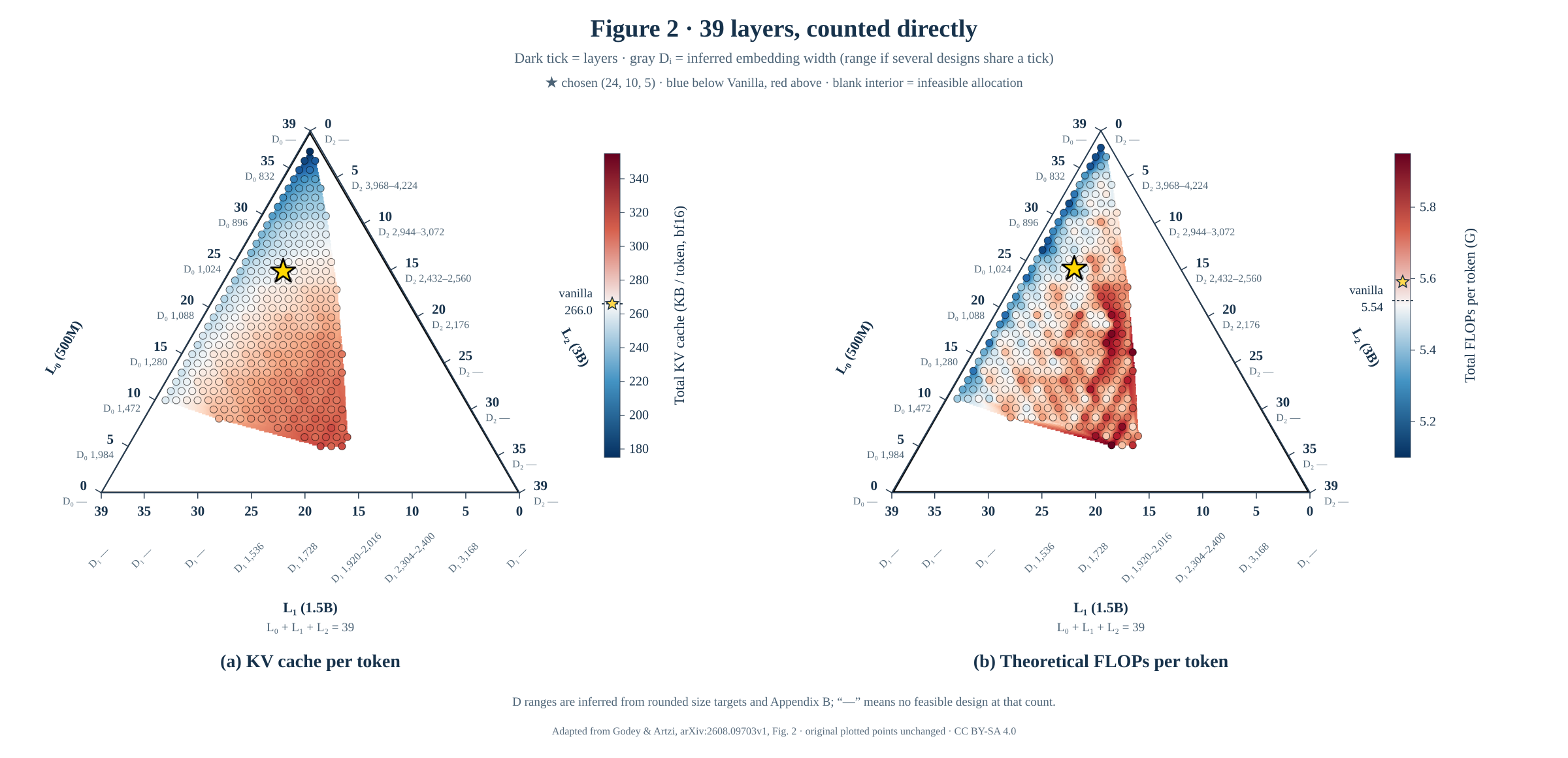
A scalable version is also available: open the SVG.

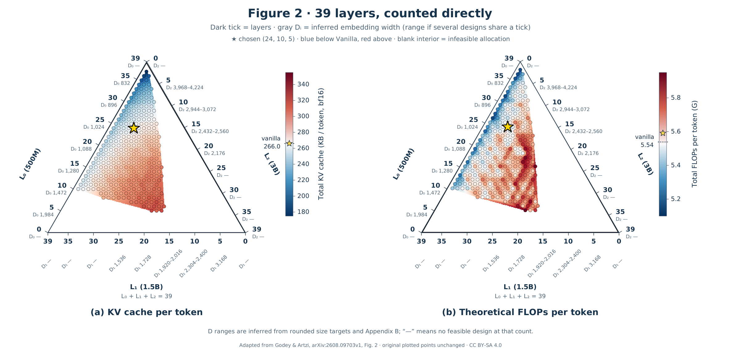
The ticks have now changed, they show not only the actualy number layers instead of a percentage that isn’t divisble by 39 easily, but they also show the possible embedding dimension throughout the model! Side L_0 still shows the 500M model, L_1 the 1.5B one and L_2 the 3B one. Near each of the number_of_layers there is a D_i number that shows the possible embedding layer dimension.

What changed and why

• Integer ticks replace fractions. Reading the fractions and might be a bit unintutive to explain the results
• Every tick has a embedding layer dimension label. The important change was the addition of the hidden embedding dimension at each nested model. The range of possible values is given by the article’s formula of Pᵢ = 2V(Dᵢ − Dᵢ₋₁) + 16LᵢDᵢ², then selecting the possible number of attention heads. The ranges can vary due to dimensions of the previous nested models (in L_1 and L_2). So, each tick shows the range! Notice that these ranges are infered mathematically and not ones that are published.

The important change is the second one and the reason is to understand why some confiugrations are not possible. The white area with no values at the 2 triangles has no explanation at the figure itself and the appendix does give the explanation but requires the reader to do manual calculations in order to check and see it for themselves. Therefore, adding the possible dimensions sizes and seeing how they decrease as the number of layers goes up (and vise versa) makes the calculation much easier, allowing the user understand how the equation of D_0<D_1<D_2 comes into play visually and intuitively. (Since no model can be narrower that its predocessor)